Creating an advanced model setup
Note
This guide is still work in progress.
This is a step-by-step guide that illustrates how even complicated setups can be created with relative ease (thanks to the tools provided by the scientific Python community). As an example, we will re-create the wave propagation setup, which is a global ocean model with an idealized Atlantic.
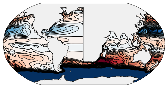
The resulting stream function after about 1 year of integration.
The vision
The purpose of this model is to examine wave propagation along the eastern boundary of the North Atlantic. Since it is difficult to track propagating waves along ragged geometry or through uneven forcing fields, we will idealize the representation of the North Atlantic; and as the presence of the Pacific in the model is crucial to achieve a realistic ocean circulation, we want to use a global model.
This leaves us with the following requirements for the final wave propagation model:
A global model with a resolution of around 2 degrees and meridional stretching.
Convert the eastern boundary of the Atlantic to a straight line, so analytically derived wave properties hold.
A refined grid resolution at the eastern boundary of the Atlantic.
Zonally averaged forcings in the Atlantic.
A somehow interpolated initial state for cells that have been converted from land to ocean in the North Atlantic.
Options for shelf and continental slope.
A multiplier setting for the Southern Ocean wind stress.
Model skeleton
Instead of starting from scratch, we can use the global one degree model as a template, which looks like this:
#!/usr/bin/env python

import os
import h5netcdf

from veros import VerosSetup, tools, veros_method, time
from veros.variables import Variable, allocate

BASE_PATH = os.path.dirname(os.path.realpath(__file__))
DATA_FILES = tools.get_assets('global_1deg', os.path.join(BASE_PATH, 'assets.yml'))


class GlobalOneDegreeSetup(VerosSetup):
    """Global 1 degree model with 115 vertical levels.

    `Adapted from pyOM2 <https://wiki.zmaw.de/ifm/TO/pyOM2/1x1%20global%20model>`_.
    """

    @veros_method
    def set_parameter(self, vs):
        """
        set main parameters
        """
        vs.nx = 360
        vs.ny = 160
        vs.nz = 115
        vs.dt_mom = 1800.0
        vs.dt_tracer = 1800.0
        vs.runlen = 0.

        vs.coord_degree = True
        vs.enable_cyclic_x = True

        vs.congr_epsilon = 1e-10
        vs.congr_max_iterations = 10000

        vs.enable_hor_friction = True
        vs.A_h = 5e4
        vs.enable_hor_friction_cos_scaling = True
        vs.hor_friction_cosPower = 1
        vs.enable_tempsalt_sources = True
        vs.enable_implicit_vert_friction = True

        vs.eq_of_state_type = 5

        # isoneutral
        vs.enable_neutral_diffusion = True
        vs.K_iso_0 = 1000.0
        vs.K_iso_steep = 50.0
        vs.iso_dslope = 0.005
        vs.iso_slopec = 0.005
        vs.enable_skew_diffusion = True

        # tke
        vs.enable_tke = True
        vs.c_k = 0.1
        vs.c_eps = 0.7
        vs.alpha_tke = 30.0
        vs.mxl_min = 1e-8
        vs.tke_mxl_choice = 2
        vs.kappaM_min = 2e-4
        vs.kappaH_min = 2e-5
        vs.enable_kappaH_profile = True
        vs.enable_tke_superbee_advection = True

        # eke
        vs.enable_eke = True
        vs.eke_k_max = 1e4
        vs.eke_c_k = 0.4
        vs.eke_c_eps = 0.5
        vs.eke_cross = 2.
        vs.eke_crhin = 1.0
        vs.eke_lmin = 100.0
        vs.enable_eke_superbee_advection = True
        vs.enable_eke_isopycnal_diffusion = True

        # idemix
        vs.enable_idemix = False
        vs.enable_eke_diss_surfbot = True
        vs.eke_diss_surfbot_frac = 0.2
        vs.enable_idemix_superbee_advection = True
        vs.enable_idemix_hor_diffusion = True

        # custom variables
        vs.nmonths = 12
        vs.variables.update(
            t_star=Variable('t_star', ('xt', 'yt', 'nmonths'), '', '', time_dependent=False),
            s_star=Variable('s_star', ('xt', 'yt', 'nmonths'), '', '', time_dependent=False),
            qnec=Variable('qnec', ('xt', 'yt', 'nmonths'), '', '', time_dependent=False),
            qnet=Variable('qnet', ('xt', 'yt', 'nmonths'), '', '', time_dependent=False),
            qsol=Variable('qsol', ('xt', 'yt', 'nmonths'), '', '', time_dependent=False),
            divpen_shortwave=Variable('divpen_shortwave', ('zt',), '', '', time_dependent=False),
            taux=Variable('taux', ('xt', 'yt', 'nmonths'), '', '', time_dependent=False),
            tauy=Variable('tauy', ('xt', 'yt', 'nmonths'), '', '', time_dependent=False),
        )

    @veros_method
    def _read_forcing(self, vs, var):
        with h5netcdf.File(DATA_FILES['forcing'], 'r') as infile:
            var = infile.variables[var]
            return np.array(var, dtype=str(var.dtype)).T

    @veros_method
    def set_grid(self, vs):
        dz_data = self._read_forcing(vs, 'dz')
        vs.dzt[...] = dz_data[::-1]
        vs.dxt[...] = 1.0
        vs.dyt[...] = 1.0
        vs.y_origin = -79.
        vs.x_origin = 91.

    @veros_method
    def set_coriolis(self, vs):
        vs.coriolis_t[...] = 2 * vs.omega * np.sin(vs.yt[np.newaxis, :] / 180. * vs.pi)

    @veros_method(dist_safe=False, local_variables=['kbot'])
    def set_topography(self, vs):
        bathymetry_data = self._read_forcing(vs, 'bathymetry')
        salt_data = self._read_forcing(vs, 'salinity')[:, :, ::-1]

        mask_salt = salt_data == 0.
        vs.kbot[2:-2, 2:-2] = 1 + np.sum(mask_salt.astype(np.int), axis=2)

        mask_bathy = bathymetry_data == 0
        vs.kbot[2:-2, 2:-2][mask_bathy] = 0

        vs.kbot[vs.kbot >= vs.nz] = 0

        # close some channels
        i, j = np.indices((vs.nx, vs.ny))

        mask_channel = (i >= 207) & (i < 214) & (j < 5)  # i = 208,214; j = 1,5
        vs.kbot[2:-2, 2:-2][mask_channel] = 0

        # Aleutian islands
        mask_channel = (i == 104) & (j == 134)  # i = 105; j = 135
        vs.kbot[2:-2, 2:-2][mask_channel] = 0

        # Engl channel
        mask_channel = (i >= 269) & (i < 271) & (j == 130)  # i = 270,271; j = 131
        vs.kbot[2:-2, 2:-2][mask_channel] = 0

    @veros_method(dist_safe=False, local_variables=[
        't_star', 's_star', 'qnec', 'qnet', 'qsol', 'divpen_shortwave', 'taux', 'tauy',
        'temp', 'salt', 'forc_iw_bottom', 'forc_iw_surface', 'kbot', 'maskT', 'maskW',
        'zw', 'dzt'
    ])
    def set_initial_conditions(self, vs):
        rpart_shortwave = 0.58
        efold1_shortwave = 0.35
        efold2_shortwave = 23.0

        # initial conditions
        temp_data = self._read_forcing(vs, 'temperature')
        vs.temp[2:-2, 2:-2, :, 0] = temp_data[..., ::-1] * vs.maskT[2:-2, 2:-2, :]
        vs.temp[2:-2, 2:-2, :, 1] = temp_data[..., ::-1] * vs.maskT[2:-2, 2:-2, :]

        salt_data = self._read_forcing(vs, 'salinity')
        vs.salt[2:-2, 2:-2, :, 0] = salt_data[..., ::-1] * vs.maskT[2:-2, 2:-2, :]
        vs.salt[2:-2, 2:-2, :, 1] = salt_data[..., ::-1] * vs.maskT[2:-2, 2:-2, :]

        # wind stress on MIT grid
        vs.taux[2:-2, 2:-2, :] = self._read_forcing(vs, 'tau_x')
        vs.tauy[2:-2, 2:-2, :] = self._read_forcing(vs, 'tau_y')

        qnec_data = self._read_forcing(vs, 'dqdt')
        vs.qnec[2:-2, 2:-2, :] = qnec_data * vs.maskT[2:-2, 2:-2, -1, np.newaxis]

        qsol_data = self._read_forcing(vs, 'swf')
        vs.qsol[2:-2, 2:-2, :] = -qsol_data * vs.maskT[2:-2, 2:-2, -1, np.newaxis]

        # SST and SSS
        sst_data = self._read_forcing(vs, 'sst')
        vs.t_star[2:-2, 2:-2, :] = sst_data * vs.maskT[2:-2, 2:-2, -1, np.newaxis]

        sss_data = self._read_forcing(vs, 'sss')
        vs.s_star[2:-2, 2:-2, :] = sss_data * vs.maskT[2:-2, 2:-2, -1, np.newaxis]

        if vs.enable_idemix:
            tidal_energy_data = self._read_forcing(vs, 'tidal_energy')
            mask = np.maximum(0, vs.kbot[2:-2, 2:-2] - 1)[:, :, np.newaxis] == np.arange(vs.nz)[np.newaxis, np.newaxis, :]
            tidal_energy_data[:, :] *= vs.maskW[2:-2, 2:-2, :][mask].reshape(vs.nx, vs.ny) / vs.rho_0
            vs.forc_iw_bottom[2:-2, 2:-2] = tidal_energy_data

            wind_energy_data = self._read_forcing(vs, 'wind_energy')
            wind_energy_data[:, :] *= vs.maskW[2:-2, 2:-2, -1] / vs.rho_0 * 0.2
            vs.forc_iw_surface[2:-2, 2:-2] = wind_energy_data

        """
        Initialize penetration profile for solar radiation and store divergence in divpen
        note that pen is set to 0.0 at the surface instead of 1.0 to compensate for the
        shortwave part of the total surface flux
        """
        swarg1 = vs.zw / efold1_shortwave
        swarg2 = vs.zw / efold2_shortwave
        pen = rpart_shortwave * np.exp(swarg1) + (1.0 - rpart_shortwave) * np.exp(swarg2)
        pen[-1] = 0.
        vs.divpen_shortwave = allocate(vs, ('zt',))
        vs.divpen_shortwave[1:] = (pen[1:] - pen[:-1]) / vs.dzt[1:]
        vs.divpen_shortwave[0] = pen[0] / vs.dzt[0]

    @veros_method
    def set_forcing(self, vs):
        t_rest = 30. * 86400.
        cp_0 = 3991.86795711963  # J/kg /K

        year_in_seconds = time.convert_time(1., 'years', 'seconds')
        (n1, f1), (n2, f2) = tools.get_periodic_interval(vs.time, year_in_seconds,
                                                         year_in_seconds / 12., 12)

        # linearly interpolate wind stress and shift from MITgcm U/V grid to this grid
        vs.surface_taux[:-1, :] = f1 * vs.taux[1:, :, n1] + f2 * vs.taux[1:, :, n2]
        vs.surface_tauy[:, :-1] = f1 * vs.tauy[:, 1:, n1] + f2 * vs.tauy[:, 1:, n2]

        if vs.enable_tke:
            vs.forc_tke_surface[1:-1, 1:-1] = np.sqrt((0.5 * (vs.surface_taux[1:-1, 1:-1] \
                                                                + vs.surface_taux[:-2, 1:-1]) / vs.rho_0) ** 2
                                                      + (0.5 * (vs.surface_tauy[1:-1, 1:-1] \
                                                                + vs.surface_tauy[1:-1, :-2]) / vs.rho_0) ** 2) ** (3. / 2.)

        # W/m^2 K kg/J m^3/kg = K m/s
        t_star_cur = f1 * vs.t_star[..., n1] + f2 * vs.t_star[..., n2]
        vs.qqnec = f1 * vs.qnec[..., n1] + f2 * vs.qnec[..., n2]
        vs.qqnet = f1 * vs.qnet[..., n1] + f2 * vs.qnet[..., n2]
        vs.forc_temp_surface[...] = (vs.qqnet + vs.qqnec * (t_star_cur - vs.temp[..., -1, vs.tau])) \
            * vs.maskT[..., -1] / cp_0 / vs.rho_0
        s_star_cur = f1 * vs.s_star[..., n1] + f2 * vs.s_star[..., n2]
        vs.forc_salt_surface[...] = 1. / t_rest * \
            (s_star_cur - vs.salt[..., -1, vs.tau]) * vs.maskT[..., -1] * vs.dzt[-1]

        # apply simple ice mask
        mask1 = vs.temp[:, :, -1, vs.tau] * vs.maskT[:, :, -1] <= -1.8
        mask2 = vs.forc_temp_surface <= 0
        ice = ~(mask1 & mask2)
        vs.forc_temp_surface *= ice
        vs.forc_salt_surface *= ice

        # solar radiation
        if vs.enable_tempsalt_sources:
            vs.temp_source[..., :] = (f1 * vs.qsol[..., n1, None] + f2 * vs.qsol[..., n2, None]) \
                * vs.divpen_shortwave[None, None, :] * ice[..., None] \
                * vs.maskT[..., :] / cp_0 / vs.rho_0

    @veros_method
    def set_diagnostics(self, vs):
        average_vars = ['surface_taux', 'surface_tauy', 'forc_temp_surface', 'forc_salt_surface',
                        'psi', 'temp', 'salt', 'u', 'v', 'w', 'Nsqr', 'Hd', 'rho',
                        'K_diss_v', 'P_diss_v', 'P_diss_nonlin', 'P_diss_iso', 'kappaH']
        if vs.enable_skew_diffusion:
            average_vars += ['B1_gm', 'B2_gm']
        if vs.enable_TEM_friction:
            average_vars += ['kappa_gm', 'K_diss_gm']
        if vs.enable_tke:
            average_vars += ['tke', 'Prandtlnumber', 'mxl', 'tke_diss',
                             'forc_tke_surface', 'tke_surf_corr']
        if vs.enable_idemix:
            average_vars += ['E_iw', 'forc_iw_surface', 'forc_iw_bottom', 'iw_diss',
                             'c0', 'v0']
        if vs.enable_eke:
            average_vars += ['eke', 'K_gm', 'L_rossby', 'L_rhines']

        vs.diagnostics['averages'].output_variables = average_vars
        vs.diagnostics['cfl_monitor'].output_frequency = 86400.0
        vs.diagnostics['snapshot'].output_frequency = 365 * 86400 / 24.
        vs.diagnostics['overturning'].output_frequency = 365 * 86400
        vs.diagnostics['overturning'].sampling_frequency = 365 * 86400 / 24.
        vs.diagnostics['energy'].output_frequency = 365 * 86400
        vs.diagnostics['energy'].sampling_frequency = 365 * 86400 / 24.
        vs.diagnostics['averages'].output_frequency = 365 * 86400
        vs.diagnostics['averages'].sampling_frequency = 365 * 86400 / 24.

    @veros_method
    def after_timestep(self, vs):
        pass


@tools.cli
def run(*args, **kwargs):
    simulation = GlobalOneDegreeSetup(*args, **kwargs)
    simulation.setup()
    simulation.run()


if __name__ == '__main__':
    run()
The biggest changes in the new wave propagation setup will be located in the
set_grid() set_topography() and set_initial_conditions()
methods to accommodate for the new geometry and the interpolation of initial
conditions to the modified grid, so we can concentrate on implementing those
first.
Step 1: Setup grid
Warning
When using a non-uniform grid,
Step 2: Create idealized topography
Usually, to create an idealized topography, one would simply hand-craft some input and forcing files that reflect the desired changes. However, since we want our setup to have flexible resolution, we will have to write an algorithm that creates these input files for any given number of grid cells. One convenient way to achieve this is by creating some high-resolution masks representing the target topography by hand, and then interpolate these masks to the desired resolution.
Create a mask image
Before we can start, we need to download a high-resolution topography dataset. There are many freely available topographical data sets on the internet; one of them is ETOPO5 (with a resolution of 5 arc-minutes), which we will be using throughout this tutorial. To create a mask image from the topography file, you can use the command line tool veros create-mask, e.g. like
$ veros create-mask ETOPO5_Ice_g_gmt4.nc
This creates a one-to-one representation of the topography file as a PNG image. However, in the case of the 5 arc-minute topography, the resulting image includes a lot of small islands and complicated coastlines that might cause problems when being interpolated to a numerical grid with a much lower resolution. To address this, the create-mask script accepts a scale argument. When given, a Gaussian filter with standard deviation scale (in grid cells) is applied to the resulting image, smoothing out small features. The command
$ veros create-mask ETOPO5_Ice_g_gmt4 --scale 3 3
results in the following mask:
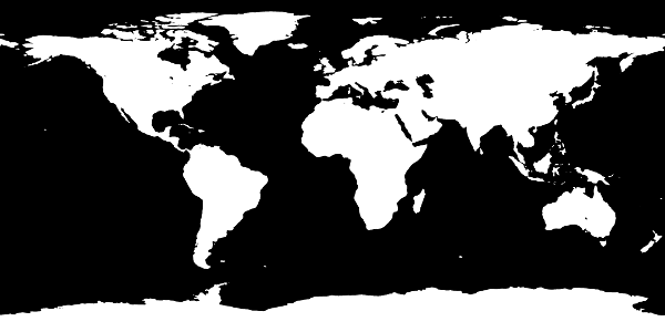
Smoothed topography mask
which looks good enough to serve as a basis for horizontal resolutions of around one degree.
Modify the mask
We can now proceed to mold this realistic version of the global topography into the desired idealized shape. You can use any image editor you have available; one possibility is the free software GIMP. Inside the editor, we can use the pencil tools to create a modified version of the topography mask:
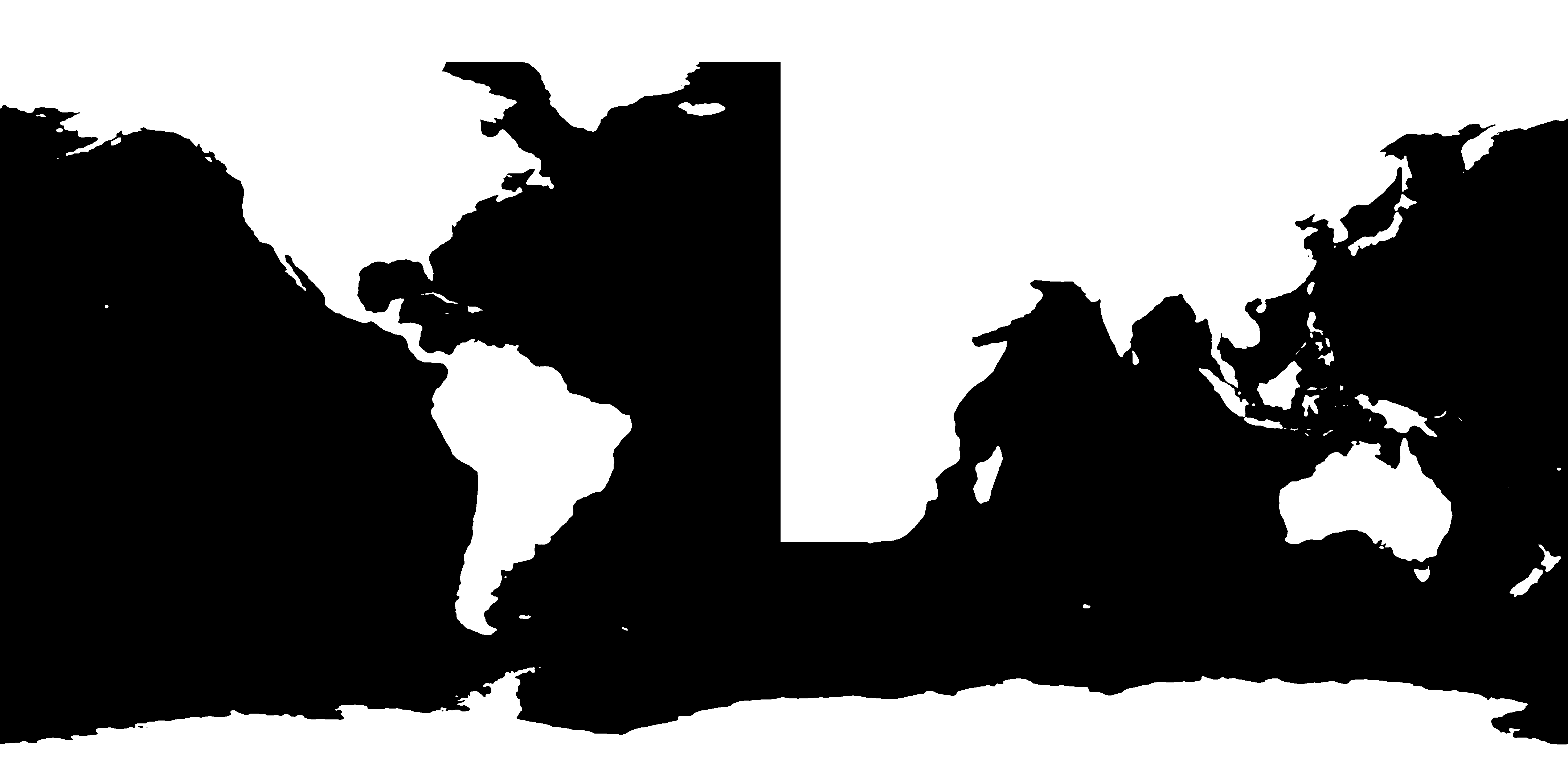
Idealized topography mask
In this modified version, I have
replaced the eastern boundary of the North Atlantic by a meridional line;
removed all lakes and inland seas;
thickened Central America (to prevent North and South America to become disconnected due to interpolation artifacts); and
removed the Arctic Ocean and Hudson Bay.
Now that our topography mask is finished, we can go ahead and implement it in the Veros setup!
Import to Veros
To read the mask in PNG format, we are going to use the Python Imaging Library (PIL).
Step 3: Interpolate forcings & initial conditions

Mask to identify grid cells in the North Atlantic