Analysis of Veros output
In this tutorial, we will use xarray and matplotlib to load, analyze, and plot the model output. We will also use the cmocean colormaps. You can run these commands in IPython or a Jupyter Notebook. Just make sure to install the dependencies first:
$ pip install xarray matplotlib h5py h5netcdf cmocean
The analysis below is performed for 100 yr integration of the global_4deg setup from the setup gallery.
If you want to run this analysis yourself, you can download the data here. We access the files through the dictionary OUTPUT_FILES, which contains the paths to the 4 different files:
In [1]: OUTPUT_FILES = {
   ...:     "snapshot": "4deg.snapshot.nc",
   ...:     "averages": "4deg.averages.nc",
   ...:     "overturning": "4deg.overturning.nc",
   ...:     "energy": "4deg.energy.nc",
   ...: }
   ...:
Let’s start by importing some packages:
In [2]: import xarray as xr

In [3]: import numpy as np

In [4]: import cmocean
Most of the heavy lifting will be done by xarray, which provides a data structure and API for working with labeled N-dimensional arrays. xarray datasets automatically keep track how the values of the underlying arrays map to locations in space and time, which makes them immensely useful for analyzing model output.
Load and manipulate averages
In order to load our first output file and display its content execute the following two commands:
In [5]: ds_avg = xr.open_dataset(OUTPUT_FILES["averages"], engine="h5netcdf")

In [6]: ds_avg
Out[6]:
<xarray.Dataset> Size: 22MB
Dimensions:       (Time: 10, yu: 40, xu: 90, zt: 15, yt: 40, xt: 90, zw: 15,
                   isle: 6, nmonths: 12, tensor1: 2, tensor2: 2)
Coordinates:
  * Time          (Time) timedelta64[ns] 80B 32760 days ... 36000 days
  * yu            (yu) float64 320B -76.0 -72.0 -68.0 -64.0 ... 72.0 76.0 80.0
  * xu            (xu) float64 720B 4.0 8.0 12.0 16.0 ... 352.0 356.0 360.0
  * zt            (zt) float64 120B -4.855e+03 -4.165e+03 ... -65.0 -35.0
  * yt            (yt) float64 320B -78.0 -74.0 -70.0 -66.0 ... 70.0 74.0 78.0
  * xt            (xt) float64 720B 2.0 6.0 10.0 14.0 ... 350.0 354.0 358.0
  * zw            (zw) float64 120B -4.51e+03 -3.87e+03 -3.28e+03 ... -50.0 0.0
  * isle          (isle) float64 48B 0.0 1.0 2.0 3.0 4.0 5.0
  * nmonths       (nmonths) float64 96B 0.0 1.0 2.0 3.0 ... 8.0 9.0 10.0 11.0
  * tensor1       (tensor1) float64 16B 0.0 1.0
  * tensor2       (tensor2) float64 16B 0.0 1.0
Data variables:
    psi           (Time, yu, xu) float64 288kB ...
    salt          (Time, zt, yt, xt) float64 4MB ...
    surface_taux  (Time, yt, xu) float64 288kB ...
    surface_tauy  (Time, yu, xt) float64 288kB ...
    temp          (Time, zt, yt, xt) float64 4MB ...
    u             (Time, zt, yt, xu) float64 4MB ...
    v             (Time, zt, yu, xt) float64 4MB ...
    w             (Time, zw, yt, xt) float64 4MB ...
Attributes:
    date_created:      2021-10-26T12:02:31.193084
    veros_version:     1.4.2
    setup_identifier:  4deg
    history:           Thu Oct 28 16:05:51 2021: ncks -d Time,90,99 4deg.aver...
    NCO:               netCDF Operators version 4.8.0 (Homepage = http://nco....
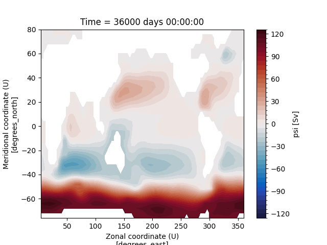
We can easily access/modify individual data variables and their attributes. To demonstrate this let’s convert the units of the barotropic stream function from \(\frac{m^{3}}{s}\) to \(Sv\):
In [7]: ds_avg["psi"] = ds_avg.psi / 1e6

In [8]: ds_avg["psi"].attrs["units"] = "Sv"
Now, we select the last time slice of psi and plot it:
In [9]: ds_avg["psi"].isel(Time=-1).plot.contourf(levels=50, cmap="cmo.balance")
Out[9]: <matplotlib.contour.QuadContourSet at 0x7d68e46c06e0>
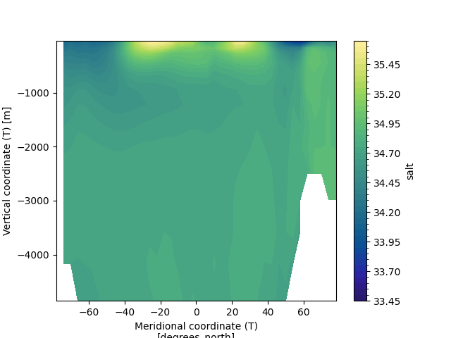
In order to compute the decadal mean (of the last 10yrs) of zonal-mean ocean salinity use the following command:
In [10]: (
   ....:     ds_avg["salt"]
   ....:     .isel(Time=slice(-10,None))
   ....:     .mean(dim=("Time", "xt"))
   ....:     .plot.contourf(levels=50, cmap="cmo.haline")
   ....: )
   ....:
Out[10]: <matplotlib.contour.QuadContourSet at 0x7d68e445c190>
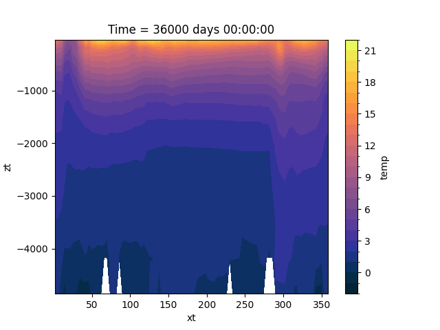
One can also compute meridional mean temperature. Since the model output is defined on a regular latitude / longitude grid, the grid cell area decreases towards the pole. To get an accurate mean value, we need to weight each cell by its area:
In [11]: ds_snap = xr.open_dataset(OUTPUT_FILES["snapshot"])

# use cell area as weights, replace missing values (land) with 0
In [12]: weights = ds_snap["area_t"].fillna(0)
Now, we can calculate the meridional mean temperature (via xarray’s .weighted method) and plot it:
In [13]: temp_weighted = (
   ....:     ds_avg["temp"]
   ....:     .isel(Time=-1)
   ....:     .weighted(weights)
   ....:     .mean(dim="yt")
   ....:     .plot.contourf(vmin=-2, vmax=22, levels=25, cmap="cmo.thermal")
   ....: )
   ....:
Explore overturning circulation
In [14]: ds_ovr = xr.open_dataset(OUTPUT_FILES["overturning"])

In [15]: ds_ovr
Out[15]:
<xarray.Dataset> Size: 4MB
Dimensions:      (Time: 100, zw: 15, yu: 40, sigma: 60, zt: 15, isle: 6,
                  nmonths: 12, tensor1: 2, tensor2: 2, xt: 90, xu: 90, yt: 40)
Coordinates:
  * Time         (Time) timedelta64[ns] 800B 360 days 720 days ... 36000 days
  * zw           (zw) float64 120B -4.51e+03 -3.87e+03 -3.28e+03 ... -50.0 0.0
  * yu           (yu) float64 320B -76.0 -72.0 -68.0 -64.0 ... 72.0 76.0 80.0
  * sigma        (sigma) float64 480B 5.804 5.934 6.064 ... 13.23 13.36 13.49
  * zt           (zt) float64 120B -4.855e+03 -4.165e+03 ... -65.0 -35.0
  * isle         (isle) float64 48B 0.0 1.0 2.0 3.0 4.0 5.0
  * nmonths      (nmonths) float64 96B 0.0 1.0 2.0 3.0 4.0 ... 8.0 9.0 10.0 11.0
  * tensor1      (tensor1) float64 16B 0.0 1.0
  * tensor2      (tensor2) float64 16B 0.0 1.0
  * xt           (xt) float64 720B 2.0 6.0 10.0 14.0 ... 346.0 350.0 354.0 358.0
  * xu           (xu) float64 720B 4.0 8.0 12.0 16.0 ... 348.0 352.0 356.0 360.0
  * yt           (yt) float64 320B -78.0 -74.0 -70.0 -66.0 ... 70.0 74.0 78.0
Data variables:
    bolus_depth  (Time, zw, yu) float64 480kB ...
    bolus_iso    (Time, zw, yu) float64 480kB ...
    trans        (Time, sigma, yu) float64 2MB ...
    vsf_depth    (Time, zw, yu) float64 480kB ...
    vsf_iso      (Time, zw, yu) float64 480kB ...
    zarea        (Time, zt, yu) float64 480kB ...
Attributes:
    date_created:      2021-10-26T12:02:33.542479
    setup_identifier:  4deg
    veros_version:     1.4.2
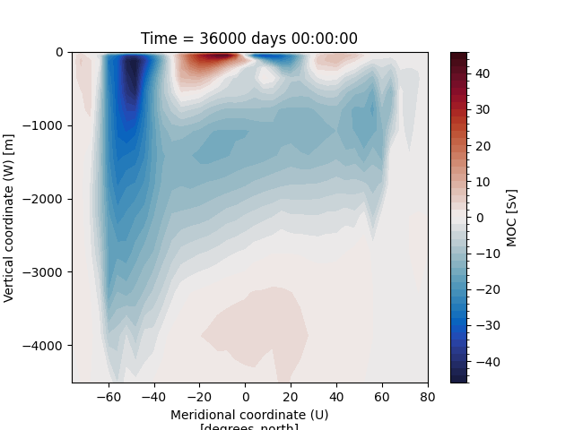
Let”s convert the units of meridional overturning circulation (MOC) from \(\frac{m^{3}}{s}\) to \(Sv\) and plot it:
In [16]: ds_ovr["vsf_depth"] = ds_ovr.vsf_depth / 1e6

In [17]: ds_ovr.vsf_depth.attrs["long_name"] = "MOC"

In [18]: ds_ovr.vsf_depth.attrs["units"] = "Sv"

In [19]: ds_ovr.vsf_depth.isel(Time=-1).plot.contourf(levels=50, cmap="cmo.balance")
Out[19]: <matplotlib.contour.QuadContourSet at 0x7d68e2027ed0>
Plot time series
Let’s have a look at the Time coordinate of the dataset:
In [20]: ds_ovr["Time"].isel(Time=slice(10,))
Out[20]:
<xarray.DataArray 'Time' (Time: 10)> Size: 80B
array([ 31104000000000000,  62208000000000000,  93312000000000000,
       124416000000000000, 155520000000000000, 186624000000000000,
       217728000000000000, 248832000000000000, 279936000000000000,
       311040000000000000], dtype='timedelta64[ns]')
Coordinates:
  * Time     (Time) timedelta64[ns] 80B 360 days 720 days ... 3600 days
Attributes:
    long_name:    Time
    time_origin:  01-JAN-1900 00:00:00
We can see that it has the type np.timedelta64, which by default has a resolution of nanoseconds. In order to have a more
meaningful x-axis in our figures, we add another coordinate “years” by dividing Time by the length of a year (360 days in Veros):
In [21]: years = ds_ovr["Time"] / np.timedelta64(360, "D")

In [22]: ds_ovr = ds_ovr.assign_coords(years=("Time", years.data))
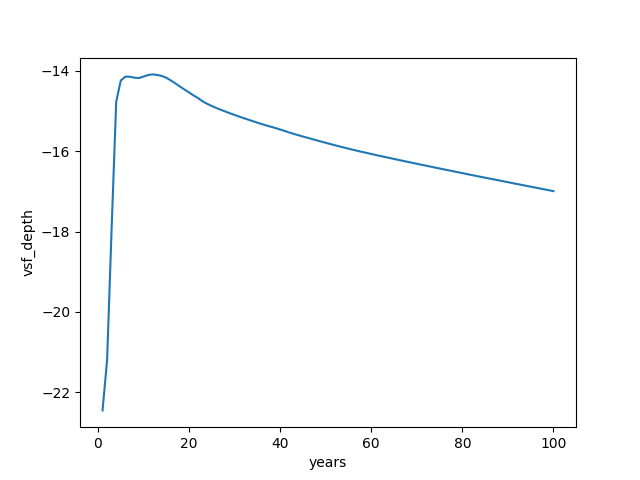
Let’s select values of array by labels instead of index location and plot a time series of the overturning minimum between 40°N and 60°N and 550-1800m depth, with years on the x-axis:
In [23]: (
   ....:     ds_ovr.vsf_depth
   ....:     .sel(zw=slice(-1810., -550.), yu=slice(40., 60.))
   ....:     .min(dim=("yu", "zw"))
   ....:     .plot(x="years")
   ....: )
   ....:
Out[23]: [<matplotlib.lines.Line2D at 0x7d68e207ea50>]